Combining OpenAI Gym with GPy - The Start
This week has been quite an exciting one; hopefully, once you have concluded reading this piece, you will feel just as excited. Having completed the task of getting used to interfacing yarp with python, my objective for the week was to bridge two python modules: OpenAI gym and GPy.
OpenAI gym is a neatly packaged module that contains within its framework different environments that simulate classical and modern problems in machine learning and intelligence. It includes problems such as the cart-pole and inverted pendulum, as well as classical atari games that you may have played quite a while ago; I sure remember them fondly! It also contains more involved simulations such as those of mobile robots. Each of these problems contain a certain goal, and OpenAI have constructed the gym framework to allow the community of machine learning to create their own algorithms and score them against other contributers according to how well achieve those goals. What’s quite extraordinary and useful about this framework is that it allows its users to access each of these environments in similar manners, requiring not much more knowledge to access one, than that needed to access another. Check the different environments that are currently available here.
GPy is a library that allows for quite easy implementations and uses of gaussian processes in python. It contains methods that allow for regression using Gaussian processes, using standard and widely used covariance kernels also manipulating them - such as summing two kernels, optimizing the hyperparameters, and more in between and beyond. Gaussian process regression, in effect, allows its user to model the inifinite number of curves that can fit a certain set of observations; it provides each of these curves with how likely they are to occur, in the form of a gaussian distribution. This gives this method phenomenal versatility and efficiency in terms of the number of observations needed in machine learning; it will be the main learning method that will be used in this project.
First Program
In order to test out how well Gaussian processes work in the problem that is described here, it was decided that GPy and OpenAI gym will be used to carry out some prelimilary analyses; since the final goal of the project is in the application of a robotic arm, the problem of the inverted pendulum was thought to be a relevant yet simple starting point.
The first program I wrote in this regard simply tried to provide controlled, yet random inputs, and extract data that can then be concatenated appropriately to be fed into a GPy regression function. The point of this was to identify the data types that each module accepted and returned, and converting between each accordingly.
In it, I am generating random control inputs within set limits of -2 to 2. Environments in OpenAI gym accept different types of data as stated in their .action_space. These can be of any dimension, continous or discrete. As an example, the Pendulum-v0 environment accepts a space called a Box which is of 1 dimension, with a highest and lowest value that can be chosen by the user.
A key point to be noted is that the function that is being fitted is the following:
where $x = x(\theta, \dot{\theta}, \ddot{\theta})$ is the state of the object, in this case the pendulum, and $u$ is the control input.
This is not a good model, and will be improved in the next program; like I said before, the point of this exercise was to simply test how a simple model can be learnt by GPy using data from OpenAI gym. Likewise, the program only learns once after a 10 tests are carried out.
Second Program
After getting that to work, I made this. The first point to be made of this program is that it forms a model of the form of:
This representation provides the model with information about how the control input in conjuction with its current state will affect the state to which it will go to; this is more realistic of a dynamic model.
Secondly, the program now trains the model at each iteration. This might not be the smartest way to go about it, but to fully appreciate how well the learning of the model takes place, learning was implented in this manner; in later exercises, I will analyse how training in batches might be more appropriate.
When running the program, the user will be asked whether the program should reset the environment at each test. Carrying out a continuous simulation, where the current state will be used as the initial conditions of the next might be a more realistic simulation; however, it is worth comparing how effective the program is when run this way, and when the state is reset to a random position at every test. The latter should provide overlapping, well to a reasonable precision of course, data points, allowing for faster learning of those points. This comparison will be shown later in this text.
The results that this program provided were both encouraging and intriguing, allowing some insight into its possible limitations, as well as those of the simulator, or rather environment in the context of this post.
Some Graphs from the Second Program
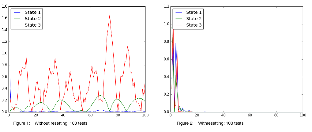
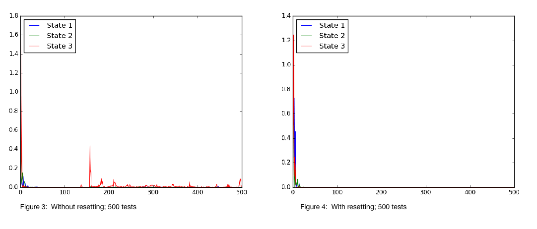
To analyse the effectiveness of the program, 5 main tests were carried out; it should have been 4, but the first test I carried might be considered a fluke, but still provided some food for thought when compared with those that followed. As I mentioned previously, there are two settings that I thought were interesting to test out: to reset, or not to. For each of these, I carried out tests that included low and high numbers of tests; these were 100 and 500 respectively. The $5^{th}$ test, or rather the $1^{st}$, was for the case of 50 tests without resetting.
Let me first prefice this by saying that there are more figures that I created from the data. Please follow this link to access them. Further, if the figures aren’t very clear, please find them in the previous link once again.
The following figures show how the absolute value of the difference between the predicted mean from the GP model and the simulation for the input parameters provided at the corresponding test; these are the y and x axes respectively.


Several observations can be made from these. The first is that resetting the states at every test allows the model to learn faster, given the input states given to it. This needs to be taken with a grain of salt however, because it is likely that the input states that are given to these experiments were limited; by allowing the simulation to be relatively continuous, the experiments that generated Figure 1 and Figure 3 most likely had a wider range of input states.
This leads on to the next observation. It appears that the error in Figure 1, and perhaps Figure 3 are increasing to begin with, but reduce as more data points are gathered. This can be explained by the fact that the control input provided causes the system to move towards states it had not encountered before, forcing the latent model to predict states in spaces it is unsure about it. However, as more tests are carried out, the simulation generates observations that overlap, improving the model’s predictability. A few anomalies occur in Figure 3, particularly in the acceleration term. This is likely due to the system encoutering accelerations that it had not encountered before.
This fact probably also explains why the error, in all 4 figures, appears to be largest in the acceleration. The acceleration term is most likely to have the largest range of values, and is also likely to be more sporadic in nature. This means that it most likely has the lowest data density, resulting in less efficient learning.
Some After Thoughts and Future Work
Please note that the analysis carried out above, and the graphs generated are by no means comprehensive. These were generated to test out the framework that was used in the program, as well as to get an intial feel for how well the program performs. In the future, more figures will be plotted to paint a better picture of what is happening; as an example, such a figure would be the time series’ of the control inputs provided and states visited.
Furthermore, I want to look at how the choice of the kernel of the GP can affect the performance of the program. Presently, the rbf model was used because it was thought that it fit the expected characteristics of the dynamical model for the pendulum; quite smooth and differentiable. This was decided upon purely qualitatively, and it might be worth refining the choice further.
It might also be worthwile looking at whether the use experimental design techniques such as the latin hypercube might be useful in this exercise; instead of randomly probing the latent space, it could be worthwile to carry out the process with more purpose.
In terms of what I will be doing next, I want to add more analysis tools to the program; this might involve the use of the RF module from last week; the RPC port can allow me to probe for information at any point during the simulation I wish, giving me more power. Furthermore, I want to generalise the program so that it can work with other environments; it might be interesting to see how the program performs in other problems.